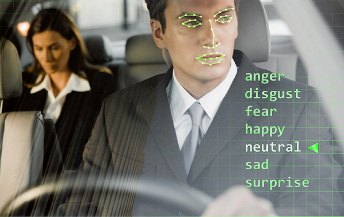
The aim of this post is to provide some numbers and recommendations after successfully fine tuning a face analysis model for a car/truck driver analysis startup. The objective was to analyse the emotions/sentiments of the drivers in a very controlled environment (a car) for inferring it’s mood. So, having an still image of the driver we need to output a basic emotion.

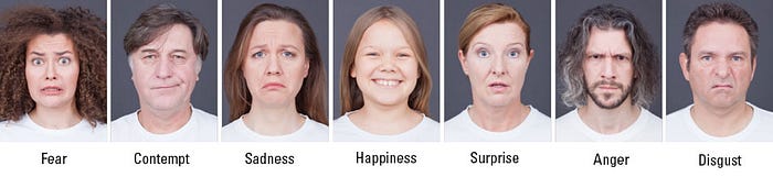
As this is a machine learning classification problem what we need are classes. In this case, we used the basic Paul Ekman emotional face expression, simple and fast.
This Ekman classification model has some problems, it does not work with transitions between emotional states (from neutral to happy) and it does not work with face expression intensities so, will a deep learning model be able to handle this problems?

As there is not enough tagged dataset available for training a deeplearning face expression model a new dataset has been build resulting in 33k images with an unbalanced classes variation. Data augmentation has been made for correcting it and resulting in two different datasets: the original and the augmented. So, I also experimented with the data necessities of the model and the results are that the effort and costs of generating new data did not pay the low accuracy augmentation of just 1 point.

Having collected the data, a preprocessing has been made before training the networks. Faces are detected with a HOG detector and then cropped. The face landmarks are detected (eyes, nose, mouth etc.) with an ensemble of regression trees. Finally the face is aligned rotating the image for obtaining an horizontal line with the eyes and their centre and then recropped as we do not want to train the models with unnecessary (for face expression analysis) data like hair or shirts.

Preprocessing is the bottleneck of the classification pipeline BUT it is essential and indispensable for having a good prediction accuracy. At this moment, we move to train the models.
The machine learning methodology known as transfer learning as been used and we looked for models trained in face recognition for importing their weights. Three architectures of convolutional neural networks had been choose:
- Alexnet, for it’s simplicity due to it’s 8 layers
- VGG16, for it’s generalisation capacities
- Resnet101, for it’s complexity with 101 layers
The three models had been trained with two datasets: the original and the augmented. So, 6 experiments had been done with the same parametrization, same computing resources, same software and data nomalization (zero mean images). We measure the results by using test (and validation) accuracy. The results are spectacular more than 95% of accuracy for each model and dataset. As I mentioned the cost of data augmentation was not necessary.


So, having such a good accuracy the dangers of overfitting threat our models. In this case the well know recommendations had been applied
- Transfer learning
- An isolated test set
- Dropout between the FC layers
- Data augmentation
Moreover, a new test set has been build with samples that are specially searched for trick the models: people with occlusions like sun glasses, beards or samples that have not been present in the training sets. No overfitting has been found but sadly, the disgraces of biased algorithms appears to us. Read more about it in this article

Thanks to Dockers containers, (with Nvidia software and Caffe) different computing resources had been used: from my simple GPU laptop to AWS and Google Cloud. In this case two GPUs had been tested: Nvidia K80 and the Pascal architecture Nvidia P100. The p100 GPU trains 4x times faster but it also cost nearly 4x times more. In this case, depending on your needs …choose a p100 GPU 🙂
So, as I had a great accuracy (from 0,94 to 0.97) I decided to share more interesting details and numbers like training times with different GPUs. With the augmented dataset of 36k images (10% validation) the fine tuning of Alexnet goes from 7 minutes in p100 to 30 minutes in k80. And with Resnet I’ve been more than 13 hours in a k80 just for recompute the last fully connected layer!

Another trade off of the three models is the weight of the model. In this case, VGG16 has been completely discarded as it has the bigger weight due the number of parameters learned 134,289,223 in front of 42,619,847 parameters that has computed the Resnet101 model. I can recommend Resnet as it has the greater generalization capacities and the best accuracy in the test set (0.977) but, if you have the needs of constantly be retraining your model in this case, the training time has to be take into consideration and then move to Alexnet.
Moving to inference, the complexity (in the number of layers) of the model has also to be take into account and in this case the differences are notable specially if you use CPU. For 742 images with a python code and Caffe framework Resnet model can take 3 hours in 4vCPUs but only 1 minute in a p100 GPU. Depending on your necessities you can deploy your technology in different ways: if you want real time you need a GPU if you can’t afford it just use offline deployment in simple CPUs

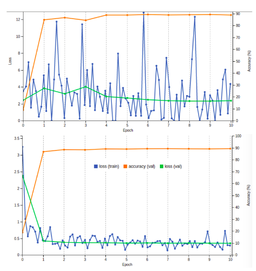
Moving to fine tuning recommendations there are two lessons learned from my project: the extreme importance of the imported weights and the only parameter to adjust that it is the learning rate (differing from the original papers parametrization). Playing with the learning rate (LR) allows you to learn in a steady and constant way that normally will converge with a great accuracy from the firsts epochs. In my case, the recommended LR is 0,001 and if you use another value your loss curves goes crazy as we can see in the following graphs.
And, the most important choice for fine tuning is the weights that you import and reuse. Fine tuning consists in reuse the learned parameters of networks with same architecture and trained for a similar purpose AND a similar dataset. In my case, I could find models pretrained for face recognition that is a classification problem trained with human faces. Everything worked smoothly. BUT, I could make some experiments with networks trained on the ImageNet dataset (1000 clases) and see with my own eyes how I could have been finish with an overfitting trained model totally incapable of generalize . Even having a 0,97 accuracy in the test set (and 0.95 in validation)! Knowing it scary me a little bit (not too much).
Networks fine tuned with imageNet weights can’t generalize in a more specific problem and for this purpose I rebuilt a new test set with samples specially searched for tricking the networks. In this case, the accuracy drop to less than 50%. But, in the case of networks finetuned with human faces weights the accuracy goes to nearly 0,9 in this trick dataset. So, you need to choose carefully your weights as there is no obvious way of detecting that you are overfitting. Well, there is a subtle difference in the train loss curves but your model can have a great test accuracy and happily deploy it but finishing with a non capable of generalize model so, a malfunctioning software.

For concluding let’s sumarise the lessons learned of this deeplearning project
- Data collection takes time. Around 70% of the time has been building a new dataset for an specific problem.
- Data preprocessing (and just 7 output classes) is the key for having a great accuracy but it only works in very environment controlled problems.
- Relatively cheap cloud resources are available in preemtible nodes or spot resources from Google cloud or AWS
- Dockers containers are the key for moving your projects around this cheap resources. Deeplearning frameworks and specially Nvidia software for working in the GPUs (CUDA and CuDnn) are very unstable and not very robust so you need to be very rigours with the software versions that you use. In this case Dockers is the perfect solution.